Line Rasters Part 1 - Brehensam

Don’t you think its fascinating how lines and circles are rendered on pixels? I’ve been wanting to implement some rasterisation algorithms in Golang. This is the 1st part of a 3 part article that deals with line rasters, their shortcomings and what has been done to improve them.

Table of Contents

• Table of Contents
• Introduction
• What’s The Problem?
• Brehensam Pseudo code and Implementation
  • Focusing on Octant 2
  • Octant 1 and 5: Gradient values between 1 and INFINITY
  • The rest of the octants: Dealing With Negativity
  • Sayonara Floating Points!
• Runtime comparison Float and Integer Implementations
• Conclusion
• Notes
• References

Introduction

Rasterization turns out to be one of those things that are really old and widely used, yet it is among one of the least understood rendering techniques among most people who rely on it daily (Yes I’m looking at you dear reader).

Perhaps let’s start by describing a problem that Rasterization solves. We draw a line from a center of one grid (point A) to another (point B). Now on a pixel display, how can we best represent lines between arbitrary points?

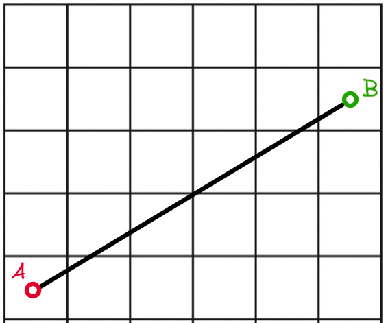
Figure 1: A simple line AB

Even if we have all the time in the world and choose to manually colorize pixels to achieve the perfectly rasterized line, we might not end up with a set of pixels that best represent the line AB.

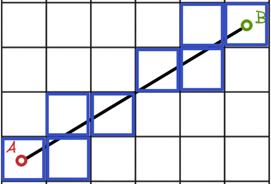
Figure 2: A manual attempt at rasterizing line AB

Let’s compare this to actually using a rasterization algorithm (Brehensam’s Line Algorithm). But the question remains: How do we know what if the rasterized result is actually the closest approximation/representation of the actual line? On what mathematical basis can we decide this?

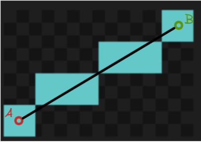
Figure 3: Line AB rasterized using Brehensam’s Algorithm

Let’s take a look at the Brehensam Line Algorithm, a classic line rasterization algorithm still in great use today. It was developed in 1962 at IBM [2] for a Calcomp Plotter.

There are plenty of articles out there explaining the Brehensam Line Algorithm and there is a particular one I like. I think he did a hella good job and I would like to build upon Colin’s work and focus on the intuition which will lead us to the algorithm.

Small note: Some articles tend to use the following coordinate frame, taking the top left as the origin (0,0), right as positive x direction, and downwards as the positive y direction.

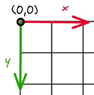
Figure 4: Image Coordinate Frame

To keep it visually intuitive. I will instead use the graph coordinate frame, and not worry about how it will translate to the image coordinate frame for now:

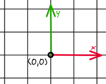
Figure 5: Graph Coordinate Frame

What’s The Problem?

The problem statement is to represent a line from point A (x1, y1) to B (x2, y2) on a grid algorithmically, whilst keeping the error between the pixels plotted and the actual line to a minimum. We make the following assumptions:

1. The start and end points coordinate are integers.
2. We will only be incrementing x as we plot the line.

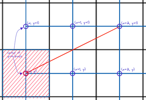
Figure 6: Problem Set up

Given the following assumption, it suffices to say that we have only 2 possible choices from which to plot. Will it be (x+1, y) in figure 7 or (x+1, y+1) in figure 8? Brehensam’s algorithm will be alternating between these 2 choices for the first octant.

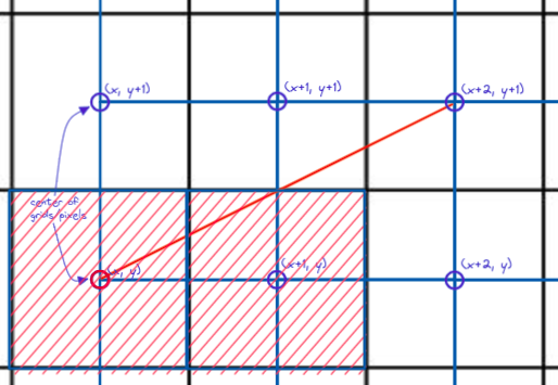
Figure 7: Do we pixelize (x+1, y)

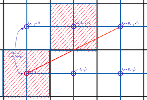
Figure 8: Or pixelize (x+1, y+1)?

However, as we start iterating through the algorithm, we will notice that the center of the plotted grid will have an error offset from the ACTUAL line. This is illustrated in figure 9.

#x1 and y1 are starting coordinates of the line
x = x1, y = y1

#Iteration 0
Actual line coordinate = (x, y)
Rasterized grid = (x, y)

#Iteration 1
Actual line coordinate = (x, y + e)
Rasterized grid = (x + 1, y)

#Iteration 2
Actual line coordinate = (x, y + e + m)
Rasterized grid = (x + 2, y + 1)

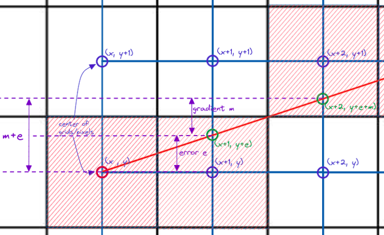
Figure 9: Error offset of y coordinate

To determine which grid to actually plot on, we have to focus on the difference between the rasterized y coordinate and the actual line y coordinate. In the example above, we will only plot on (x+2, y+1) if:

y + e + m >= y + 0.5

Similarly, we will only plot on (x+2, y) if:

y + e + m < y + 0.5

After plotting on each increment of x, we notice that now the error has changed, and how the error changes depends on whether we pick (x+2, y+1) or (x+2, y). If we pick (x+2, y+1), the new error is now:

e_new = (y + e_old + m) - (y + 1)

e_new = e_old + m - 1

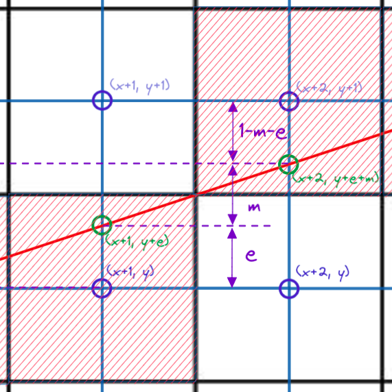
Figure 10: New error for picking (x+2, y+1)

If we pick (x+2, y), the new error is now:

e_new = (y + e_old + m) - (y)

e_new = e_old + m

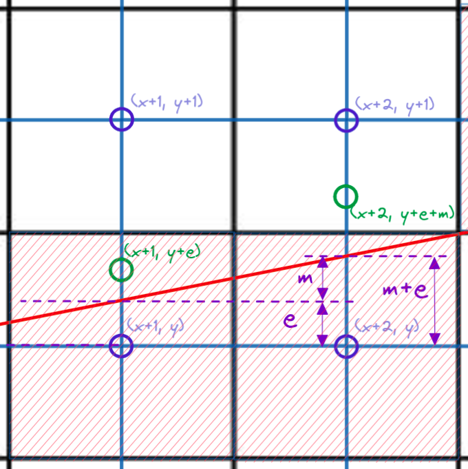
Figure 11: New error for picking (x+2, y)

Take note that the error always takes reference from the y coordinate of the currently chosen grid!

Brehensam Pseudo code and Implementation

Focusing on Octant 2

With the preceding concepts in place, we are ready to form our pseudo code:

# Set error to zero
e = 0 
# Calculate gradient
m = (y2 - y1)/(x2 - x1)

y = y1

FOR x = x1 to x2
    CALL plot(x,y)
    IF ( e + m < 0.5)
        # Increment error by m (error offset taken from y)
        e += m
    ELSE 
        y += 1
        # Increment error by m but error offset taken from y+1
        e += m -1
    END IF
END FOR

Code Block 1: Brehensam’s Line Algorithm for Octant 2 Pseudo code

You can try implementing the above in your favorite programming language, but for now let’s try implementing this in Golang!

//GOLANG IMPLEMENTATION

m := (float64(y2 - y1)) / (float64(x2 - x1)) //calculate gradient

for x, y, err := x1, y1, 0.0; x != x2+1; x += 1 {
    // Plot point (x,y)
    img.Set(x, y, color)
    if (err + m) < 0.5 {
        // Increment error by m (error offset taken from y)
        err += m
    } else {
        y += 1
        // Increment error by m but error offset taken from y+1
        err += m - 1
    }
}

Code Block 2: Code Block 1 implemented in GOLang

We will choose to draw a 12 pointed star (Figure 12) to demonstrate that Brehensam is able to handle all signs and magnitude of gradients, by passing in the following input, which will be parsed as x1, y1 -> x2, y2

8,8 -> 4,0; 
8,8 -> 0,4; 
8,8 -> 12,0;
8,8 -> 16,4;
8,8 -> 16,12;
8,8 -> 12,16;
8,8 -> 4,16;
8,8 -> 0,12;
8,8 -> 8,0;
8,8 -> 0,8;
8,8 -> 8,16;
8,8 -> 16,8;

Code Block 3: Input given to my programme

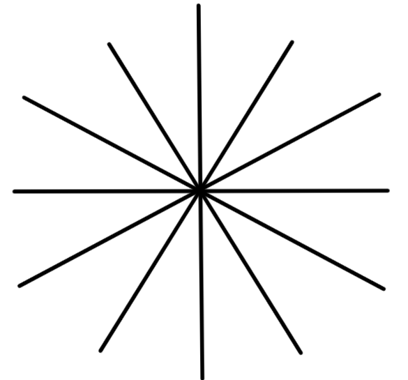
Figure 12: 12 pointed star

But wait… running our algorithm now will simply put us in an infinite loop where both x and y and incremented, which means that for some lines, (err + m) will always be more than or equal to 0.5

Turns out our pseudo code only applies for the second octant, which is highlighted in figure 14. Our current algorithm is only able to handle positive gradient values between 1 and 0.

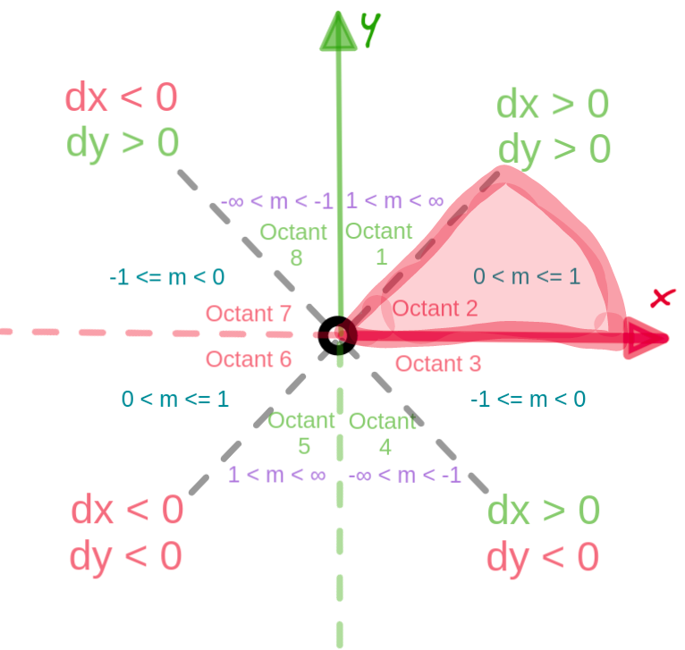
Figure 14: Octant 2 is highlighted here among the other octants

Octant 1 and 5: Gradient values between 1 and INFINITY

Lets solve for the case that we have a positive gradient value between 1 and infinity. There will be a few small changes made to the algorithm:

1. We will need to set the new gradient value as the reciprocal of the actual line gradient.
2. Iterate y from y1 to y2 (Instead of iterating through x)

e = 0 
# Calculate reciprocal of gradient
m = (x2 - x1)/(y2 - y1)

x = x1

FOR y = y1 to y2
    CALL plot(x,y)
    IF ( e + m < 0.5)
        e += m
    ELSE 
        x += 1
        e += m -1
    END IF
END FOR

__Code Block 4: Brehensam pseudo code octant 1 __

The rest of the octants: Dealing With Negativity

We can use the easy trick of swapping the end and start points of the line, to make the gradient positive, but this means that we are going to be tracing our line from the end point to the start point and it feels like kinda cheap. Let’s try another way around it.

#...

FOR x = x1 to x2
    CALL plot(x,y)
    IF ( e + m > -0.5)
        e += m
    ELSE 
        y += 1
        e += m + 1
    END IF
END FOR

__Code Block 5: Brehensam Pseudo code Octant 3 __

This can similarly be applied to gradient values where -INFINITY < m < 1.

Now, we can reduce the pseudo code above to as little lines as possible and implement this in golang:

	dx, dy := x2-x1, y2-y1

	grad_sign := 1.0                  //Sign of gradient
	if bool(dx < 0) != bool(dy < 0) { // (dx is negative) XOR (dy is negative)
		grad_sign = -1.0
	}

	//We use x_inc and y_inc to either increment or decrement x or y depending on the sign of the gradient
	x_inc := line_render.CopySignInt(1, dx)
	y_inc := line_render.CopySignInt(1, dy)

	var m float64
	if dx != 0 { //Only calculate gradient if it is not infinite
		m = (float64(dy)) / (float64(dx)) //gradient
	}
	if line_render.Abs(dy) > line_render.Abs(dx) { // if absolute value of gradient > 1, then invert it
		m = 1 / m
	}

	if dx == 0 && dy == 0 {
		fmt.Printf("Start and end coordinates are the same \n")
		return
	} else if dx == 0 { // m == INF
		for y := y1; y != y2+y_inc; y += y_inc {
			img.Set(x1, y, color)
		}
	} else if dy == 0 { // m == 0
		for x := x1; x != x2+x_inc; x += x_inc {
			img.Set(x, y1, color)
		}
	} else if line_render.Abs(dy) > line_render.Abs(dx) { // 1 < abs(m) < INF
		// fmt.Printf("1st, 5th, 4th and 8th Octant: 1 < abs(m) < INF \n")
		for x, y, err := x1, y1, 0.0; y != y2+y_inc; y += y_inc {
			img.Set(x, y, color)
			if grad_sign*(err+m) < 0.5 {
				err += m
			} else {
				err += m - grad_sign*1
				x += x_inc
			}
		}
	} else { // 0 < abs(m) <= 1
		// fmt.Printf("2nd, 6th, 3rd and 7th Octant: 0 < abs(m) <= 1 \n")
		for x, y, err := x1, y1, 0.0; x != x2+x_inc; x += x_inc {
			img.Set(x, y, color)
			if grad_sign*(err+m) < 0.5 {
				err += m
			} else {
				err += m - grad_sign*1
				y += y_inc
			}
		}
	}

Code Block 6: Golang Implementation of Brehensam Float

With this code, we are poised to form our 12 pointed star using the input from Code Block 3.

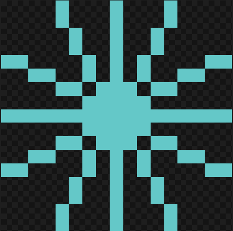
Figure 15: 12 Pointed Star Rasterized

Sayonara Floating Points!

So far everything we have talked about involves floating point operations, but that can be the bane of all evil when it comes to efficiency. So naturally we would want to simplify it to only perform integer based operations.

The following equations will be further massaged to get rid of the floating point variable m:

e + m < 0.5 (1)

e = e + m (2)

e = e + m - 1 (2)

For equation (1), we will multiply both sides by dx, where dx = x2 - x1:

e + m < 0.5 (1)

(e + m) * dx < 0.5 * dx

(e + (dy/dx)) * dx < 0.5 * dx

2e * dx + 2dy < dx

2(e’ + dy) < dx (_where e’ = edx_)

e * dx + dy < 0.5 * dx (4)

For equation (2), we also multiply both sides by dx:

e = e + m (2)

e * dx = (e + m) * dx

e’ = e’ + dy (5)

For equation (3), the same thing:

e = e + m - 1 (3)

e’ = e’ + dy - dx (6)

Now our new pseudo code for octant 2 becomes:

e = 0 
y = y1
dy = y2 - y1
dx = x2 - x1

FOR x = x1 to x2
    CALL plot(x,y)
    IF ( 2(e' + dy) < dx)
        # Increment error by m (error offset taken from y)
        e' += dy
    ELSE 
        y += 1
        # Increment error by m but error offset taken from y+1
        e' += dy - dx
    END IF
END FOR

Code Block 7: Brehensam Integer Version (Octant 2) Pseudo code

Implementing this in Golang…

    dx, dy := x2-x1, y2-y1

    grad_sign := 1                    //Sign of gradient
    if bool(dx < 0) != bool(dy < 0) { // (dx is negative) XOR (dy is negative)
        grad_sign = -1
    }
    x_inc := line_render.CopySignInt(1, dx)
    y_inc := line_render.CopySignInt(1, dy)

    if dx == 0 && dy == 0 {
        fmt.Printf("Start and end coordinates are the same \n")
        return
    } else if dx == 0 { // m == INF
        for y := y1; y != y2+y_inc; y += y_inc {
            img.Set(x1, y, color)
        }
    } else if dy == 0 { // m == 0
        for x := x1; x != x2+x_inc; x += x_inc {
            img.Set(x, y1, color)
        }
    } else if line_render.Abs(dy) > line_render.Abs(dx) { // 1 < abs(m) < INF
        // fmt.Printf("1st, 5th, 4th and 8th Octant: 1 < abs(m) < INF \n")
        for x, y, err := x1, y1, 0; y != y2+y_inc; y += y_inc {
            img.Set(x, y, color)
            if grad_sign*2*(err+dx) < dy {
                err += y_inc * (dx)
            } else {
                err += y_inc * (dx - (grad_sign * dy))
                x += x_inc
            }
        }
    } else { // 0 < m <= 1
        // fmt.Printf("2nd, 6th, 3rd and 7th Octant: 0 < abs(m) <= 1 \n")
        for x, y, err := x1, y1, 0; x != x2+x_inc; x += x_inc {
            img.Set(x, y, color)
            if grad_sign*2*(err+dy) < dx {
                err += x_inc * (dy)
            } else {
                err += x_inc * (dy - (grad_sign * dx))
                y += y_inc
            }
        }
    }

Code Block 8: Golang Implementation of Brehensam Integer

Note: If we are going to plot on images, we need to use the image coordinate frames Figure 4 instead of Figure 5. This means that the octant model in Figure 14 will be flipped vertically as shown in Figure 16.

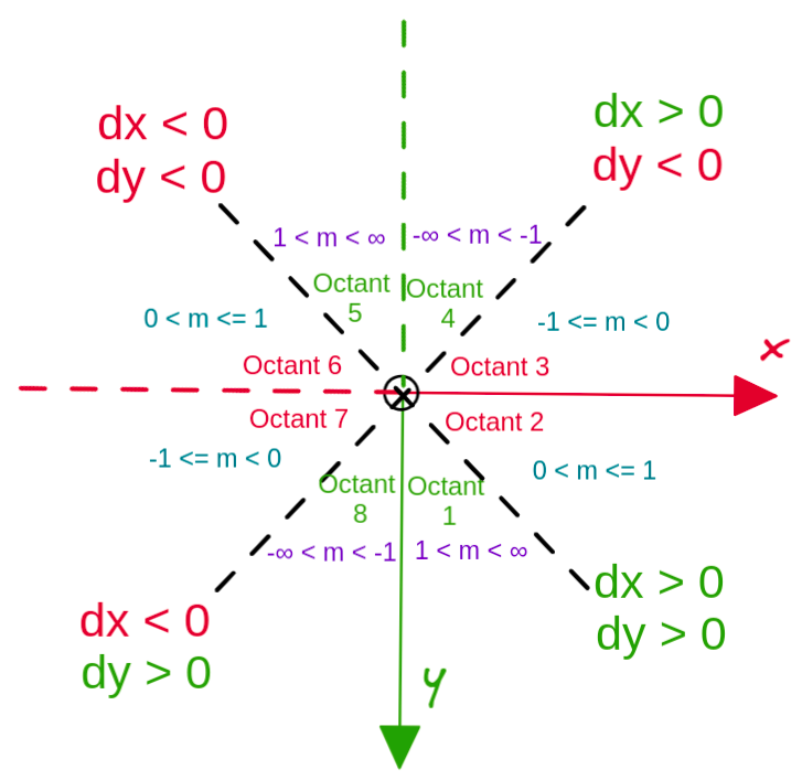
Figure 16: Flipped Octant model for image coordinate frame

Runtime comparison Float and Integer Implementations

Now let’s do some “dirty” comparison by utilizing simple timers in our code segments.

We shall draw a nice little house (The only one I might be able to afford given the housing situation in Singapore), and compare the time required to draw it using the integer and floating point version of Brehensam (Code block 6 and 8 respectively).

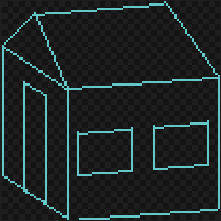
Figure 17: Our little Raster House

0,20 -> 15,5; 1
15,5 -> 30,40; 2
30,40 -> 0,20; 3
0,20 -> 0,80; 4
0,80 -> 30,100; 5
30,100 -> 30,40; 6
30,40 -> 100,35; 7
100,35 -> 100,95; 8
100,95 -> 30,100; 9
100,35 -> 75,0; 10
75,0 -> 15,5; 11
10,87 -> 20,93; door 1
20,93 -> 20,43; door 2
20,43 -> 10,37; door 3
10,37 -> 10,87; door 4
35,80 -> 60,78; window a1
60,78 -> 60,58; window a2
60,58 -> 35,60; window a3
35,60 -> 35,80; window a4
70,77 -> 95,75; window b1
95,75 -> 95,55; window b2
95,55 -> 70,57; window b3
70,57 -> 70,77; window b4

Code Block 9: Input used to draw house

Upon timing both implementations, we can see that the integer implementation does outperform the float implementation although seemingly not by much, but that might be because we did not use large data input sizes.

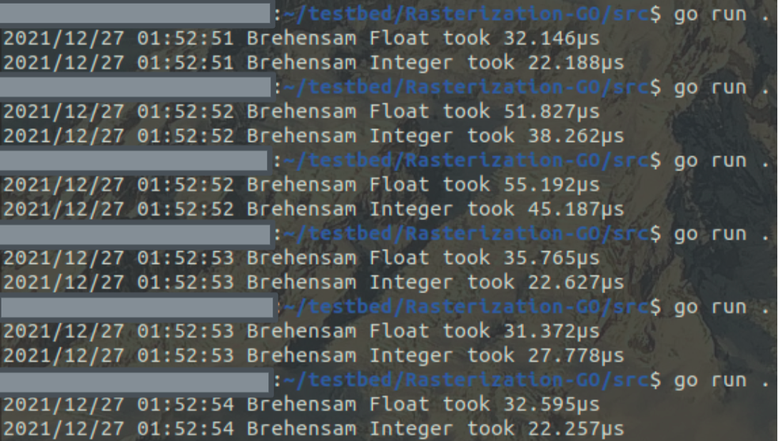
Figure 17: Comparison in elapsed run time between integer and float implementation

Conclusion

Although Brehensam’s algorithm fast and simple implementation has led to it’s importance in many graphics library and even in the firmware of graphics card, there are numerous issues that it is not made to address.

Namely, there is an aliasing effect for lines drawn using this algorithm. The lines appear jagged up close and people do get sick of retro-looking graphics after a while. This issue is solved by Xiaolin Wu’s Line Algorithm, which performs anti-aliasing and handles cases where the endpoints of the line do not lie exactly on integer points of the pixel grid [3]. We will take a look at Wu’s algorithm in Part 3.

Secondly, we have not seen how Brehensam’s Line Algorithm is able to raster curves, and that will be the focus of Part 2.

Notes

• The source code for my Golang rasterization program can be found here
• Diagrams were made with excalidraw
• I tried to follow [4] for the pseudo code syntax.
• I have been trying to learn markdown formatting properly and this guide helped me tremendously.
• Please let me know if there are any inconsistencies or misstated facts at john_tanguanzhong@hotmail.com

References

[1] Brehensam’s Line Algorithm Pseudo code

[2] Paul E. Black. Dictionary of Algorithms and Data Structures, NIST.

[3] Wikipedia Entry for Xiaolin Wu’s Line Algorithm

[4] An Introduction to Writing Good Pseudo code